HBaseWD and HBaseHUT: Handy HBase Libraries Available in Public Maven Repo

HBaseWD is aimed to help distribute writes of records with sequential row keys in HBase (and avoid RegionServer hotspotting). Good introduction can be found here.

We recently published 0.1.0 version of the library to Sonatype public maven repository. Thus, integration in your project became much easier:

  <repositories>
    <repository>
      <id>sonatype release</id>
      <url>https://oss.sonatype.org/content/repositories/releases/</url>
    </repository>
  </repositories>
  <dependency>
    <groupId>com.sematext.hbasewd</groupId>
    <artifactId>hbasewd</artifactId>
    <version>0.1.0</version>
  </dependency>

HBaseHUT is aimed to help in situations when you need to update a lot of records in HBase in read-modify-write style. Good introduction can be found here.

We recently published 0.1.0 version of this library to Sonatype public maven repository too. Integration info:

  <repositories>
    <repository>
      <id>sonatype release</id>
      <url>https://oss.sonatype.org/content/repositories/releases/</url>
    </repository>
  </repositories>
  <dependency>
    <groupId>com.sematext.hbasehut</groupId>
    <artifactId>hbasehut</artifactId>
    <version>0.1.0</version>
  </dependency>

For running (MR jobs) on hadoop-2.0+ (which is a part of CDH4.1+) use 0.1.0-hadoop-2.0 version:

  <dependency>
    <groupId>com.sematext.hbasehut</groupId>
    <artifactId>hbasehut</artifactId>
    <version>0.1.0-hadoop-2.0</version>
  </dependency>

Thank you to all contributors and users of the libraries!

Locating Mountains and More with Mahout and Public Weather Dataset

Recently I was playing with Mahout and public weather dataset. In this post I will describe how I used Mahout library and weather statistics to fill missing gaps in weather measurements and how I managed to locate steep mountains in US with a little Machine Learning (n.b. we are looking for people with Machine Learning or Data Mining backgrounds – see our jobs).

The idea was to just play and learn something, so the effort I did and the decisions chosen along with the approaches should not be considered as a research or serious thoughts by any means. In fact, things done during this effort may appear too simple and straightforward to some. Read on if you want to learn about the fun stuff you can do with Mahout!

Tools & Data

The data and tools used during this effort are: Apache Mahout project and public weather statistics dataset. Mahout is a machine learning library which provided a handful of machine learning tools. During this effort I used just small piece of this big pie. The public weather dataset is a collection of daily weather measurements (temperature, wind speed, humidity, pressure, &c.) from 9000+ weather stations around the world.

Artificial Problems

The problems I decided to attack (I made up them by myself, just to set some goals, no serious research was intended) were

  • using Mahout’s recommendation tools to fill the missing data points in weather statistics data
  • using Mahout’s “similarity tools” to locate nature’s relief influencers on the weather conditions, like mountains, based on weather statistics data

First would allow to fill in gaps in measurements on some of the weather stations. In the second problem the system would locate physical nature’s barriers and other influencers on the weather. By comparing the findings with the physical map one could judge e.g. about which mountains can isolate weather spreading to certain areas. Please forgive me if I use the wrong terms, but I really find the outcome quite interesting. Read on!

Using Recommendation Engine to Fill Missing Weather Measurements

The core (simple) idea is to use recommendation engine to fill in missing measurements. I used User-based recommendation specifically by treating station as a user, date as an item and the temperature as a preference. I know, many can say this isn’t a good way to approach the problem, but for my purpose of learning this worked well.

The Data

The dataset contains 18 surface meteorological elements, from which I selected just few items to be used. So, I chose to work only with temperature to simplify things, though I understood that it could not be enough to reach any interesting result. Moreover, one would argue that it makes much more sense to use precipitation to locate such objects as mountains which affect them a lot. I chose a simpler path, though with quite a big risk of getting nothing. In order to have ability to iterate fast I also used just 2 years of data of the stations located in US. I actually tried to use only California’s station, but this didn’t work well (at least in the beginning before I get to tuning the system logic). For this first problem I didn’t use any of the stations location and altitude information to get things more interesting.

To evaluate the system I simply divided the dataset into two pieces and used one of each as training sample and another one as evaluation sample. Please see the code below.

Data Cleaning

I had to clean some the data before I could use it for training the recommender. It seems like there were some stations which has different IDs but has same location in the dataset. I cleaned them to have only one station in the same place to avoid increased weighting of the same station. I also cleaned Alaska’s stations and most of those which are not on the continental area as they are usually alone standing and do not have related weather conditions to others and only bring the noise for the recommender.

Preparing Input Data for Mahout

So, in our interpretation stations are users and days (dates) with temperature are items with user preference, but there’s more to that. It makes sense to try to use connection between dates which is just dropped by this simple interpretation: dates may stand close to each other or be far from each other; by comparing the change of the temperature during some period helps to judge about “weather closeness” of two stations. To make use of that for calculating similarity I also added <date, diff with the N days ago> pairs. E.g. for input:

20060101,56
20060102,61
20060103,62

I got these preferences:

20060101_0,56
20060102_0,61
20060102_1,+5/1
20060103_0,62
20060103_1,+1/1
20060103_2,+6/2

I divided the difference with the further standing “N day ago” by N so that they are weighted less. Otherwise difference between far from each other days going to be bigger than from than that from close days, while it is the close days difference which is more interesting actually. For the same purpose I tested with up to 5 extra pairs (diffs with up to 5 previous days).

Moreover, when it comes to comparing the change it may really not matter by how much temperature was changed, it is enough to know that it was changed at least by some value d (onlyDirectionOfChange=true, changeWeight=d in results below). So, e.g. given value d=2.0, comparing change with previous 2 days (prevDays=2 in the results below) the example data above is going to look like this:

20060101_0,56
20060102_0,61
20060102_1,+2/1
20060103_0,62
20060103_1,0
20060103_2,+2/2

Running Recommender Evaluating Results

Once data is prepared and you know which recommender parameters (including similarities and their parameters and such) training recommender and evaluating the results is very simple. Please find below the code for non-distributed recommendation calculation.

DataModel model = new FileDataModel(statsFile);
RecommenderEvaluator evaluator = new AverageAbsoluteDifferenceRecommenderEvaluator();
RecommenderBuilder builder = new RecommenderBuilder() {
  @Override
  public Recommender buildRecommender(DataModel model) throws TasteException {
    UserSimilarity similarity = new EuclideanDistanceSimilarity(model);
    UserNeighborhood neighborhood = new NearestNUserNeighborhood(neighbors, similarity, model);
    Recommender recommender = new GenericUserBasedRecommender(model, neighborhood, similarity);
    return recommender;
  }
};
return evaluator.evaluate(builder, null, model, 0.95, 1.0);

The code above shows just one of many possible recommender configurations (and it doesn’t show the fact that we use more data for calculating user similarity as explained in the previous section). Since we really care about the numbers we throw away similarities that don’t take into account the preference value, like TanimotoCoefficientSimilarity. During the (limited) tests I ran it appeared that the simplest EuclideanSimilarity worked best.

Result

My (limited) tests showed the following best results with configurations:

SCORE: 2.03936; neighbors: 2, similarity: {onlyDirectionOfChange=true, changeWeight=2.0, prevDays=1}
SCORE: 2.04010; neighbors: 5, similarity: {onlyDirectionOfChange=true, changeWeight=5.0, prevDays=2}
SCORE: 2.04159; neighbors: 2, similarity: {onlyDirectionOfChange=false, prevDays=1}

Where:

  • “score” is the recommendation score, i.e. in our case the average absolute difference in recommended value and actual value
  • “neighbors” is the number of neighbors used (in NearestNUserNeighborhood) to provide recommendation
  • “onlyDirectionOfChange” is whether we use absolute change value when comparing with previous days (value is false) or we comparing with the certain threshold as explained above (value is true)
  • “changeWeight” is the threshold to compare the change with
  • “prevDays” is the number of previous days to compare with

Using Statistics-based Similarity to Locate Weather Influencers

The core (simple) idea is to calculate similarity between stations based on weather statistics and compare it with the physical distance between the stations: if there’s a great difference then assume that there’s something in between such stations that makes the weather noticeably different. Then, the only things we need to define is:

  • how to calculate similarity
  • haw to calculate physical distance
  • what is a *noticeable* difference between weather stats based similarity and physical distance
  • where is this “in between” located

The plan was to use Mahout’s user similarities to calculate the distance between stations based on weather statistics data (taking it as user preferences similar to the first part) and compare it with the physical distance. The evaluation of the results is not very well automated as in previous part, though it could be have I more time for this. To evaluate I just plotted the results and compared this image with the physical map of US.

The Data

The data was used the same as was used in the first part plus physical location of the station, which was used to calculate physical distance between them.

Data Cleaning

Data cleaning had the same logic as for the first part. Though I did more severe cleaning of stations not on the continent and near the shore: we all know that ocean influences the weather a lot, so if I didn’t do that, all shore points would have been considered to be “outliers”. Actually, not only ocean shore-close stations, but most of those near the border of US were removed for the sake of removal algorithm simplicity.

Preparing Input Data for Mahout

The input data were prepared the same way as in first part, the “user preferences” contained <station, temperature> pairs and added <date, diff with the N days ago> pairs. Note, that there are a lot of ways to calculate distance between stations using weather stats, I simply chose the one which would allow me to re-use the same prepared data files from the first part of experiment.

Running the Implementation & Evaluating Results

Let’s have a closer look at how each item from the list in idea overview section was defined.

How to calculate similarity?

As mentioned above I chose simple (similar to the first part) similarity calculation. Simple EuclideanDistanceSimilarity worked well.

How to calculate physical distance?

Physical distance was calculated as Euclidean distance between stations using latitude, longitude and altitude. The longitude was given a much greater weight, because the temperature tends to be affected a lot by longitude coordinate: the further South you go (in Northern Hemisphere where US is) the lower the temperature without any physical relief influencers. Also altitude was given a stronger weight because it has the same strong affect on the temperature.
And, of course to make distance comparable with calculated similarity we need it to be in 0..1 range (with the value close to 1 showing the smallest distance). Hence distance was calculated as 1 / (1 + phys_dist(station1, station2)).

What is a *noticeable* difference between weather stats based similarity and physical distance?

I assumed that there’s an exponential dependency between calculated physical distance of the two stations and similarity calculated from weather stats. I found an average growth rate (of the similarity given the physical distance) using all stations pairs (remember that we have not huge amount of stations, so we can afford that) and used it to detect those pairs that had much greater difference between their physical distance and similarity calculated from weather stats.

Where is this “in between” located?

For those “outlier” pairs detected I put single “physical influencer” point on the map which location is exactly the middle point between those stations (unweighted latitude and longitude were used to calculate it).

Result

Result is better represented and evaluated by comparing the following two images: first created by our system and second being a physical map of US.

red – cleaned “far standing” stations
green – stations which stats were used
blue – found weather “influencers”
circles – some of the cities (Seattle, San-Francisco, Los-Angeles, San-Antonio, Salt Lake City, Miami, New York City, Boston, Chicago)

Compare with:

Note how steep mountains are there in the first image. Of course, there’s noise from lakes, gulfs and other sources. But look how well it drew the relief of California!

What Else?

There are a number of things that can be done to obtain even more interesting results. Just to name a few:
* use not only temperature but other measures, e.g. precipitation as noted in the beginning of the post
* show influencers with different color (heat map) depending on how they affect the weather
* and more

Summary

I touched only a very small piece of the great collection of machine learning tools offered by Mahout and yet managed to get very interesting (and useful?) results. I also used just a small part of the public weather dataset available to everyone and yet it was enough to get meaningful outcome. And there are so many different public datasets available online! There’s so much exciting things one can do with such a powerful tool like Mahout and a pile of data.

@abaranau

HBase FuzzyRowFilter: Alternative to Secondary Indexes

In this post we’ll explain the usage of FuzzyRowFilter which can help in many situations where secondary indexes solutions seems to be the only choice to avoid full table scans.

Background

When it comes to HBase the way you design your row key affects everything. It is a common pattern to have composite row key which consists of several parts, e.g. userId_actionId_timestamp. This allows for fast fetching of rows (or single row) based on start/stop row keys which have to be a prefix of the row keys you want to select. E.g. one may select last time of userX logged in by specifying row key prefix “userX_login_”. Or last action of userX by fetching the first row with prefix “userX_”. These partial row key scans work very fast and does not require scanning the whole table: HBase storage is optimized to make them fast.

Problem

However, there are cases when you need to fetch data based on key parts which happen to be in the middle of the row key. In the example above you may want to find last logged in users. When you don’t know the first parts of the key partial row key scan turns into full table scan which might be very slow and resource intensive.

Possible Solution #1: Data Redundancy

One possible way around it would be to use secondary indexes by creating redundant rows with the same data as original ones but with different sequence of the parts of the key (e.g. actionId_timestamp). This solution may not be suitable for some because of its cons:

  • storing extra indexes (usually it requires to store N times more data for N indexes) results in storing a lot more data on disk
  • storing (and serving) extra rows brings additional load on the cluster during writing and reading (extra blocks fighting to be in cache, etc.)
  • writing/updating/deleting several rows is not an atomic operation in HBase

Possible Solution #2: Integrated Secondary Indexes

Another way to attack the problem is to use smart secondary indexes mechanism integrated in HBase which doesn’t rely on data redundancy. E.g. something like IHBase. The problem here is that there’s no out-of-the box solution to be used. This may change with addition of newer CoProcessors functionality (see e.g. HBASE-2038 or this). But as of now existent solutions have their own limitations and drawbacks while new solutions are yet to be completed.

Suggested Solution

First of all, I have to say that solution suggested below is not a silver bullet. Moreover its performance may be very bad and even be close to full table scan in some cases. Even more: it can’t be used in any of the situations described in Background and Problem sections. But in many cases depending on your data the suggested simple solution can be used to avoid secondary indexes burden and still allow for very fast scans. In many other cases it can be used to significantly speed up your full table scans.

Suggested solution is not new and quite simple, but it is usually overlooked by HBase users, though it shouldn’t be.

Fast-Forwarding in Server-side Filter

In recent HBase versions (I believe in 0.90.+) there’s a mechanism that allows skipping the whole range of rows when scanning with server-side filter. These skipped rows data may not even be read from the disk. Based on the current row key the filter can tell scanner to advance to the row with the specific key and by doing that jump over many rows which are simply skipped. For example, this makes it possible to perform fast full-table scans (or large partial key scans) in case there’s enough information about the key and the data that allows to provide efficient hints for skipping a lot of rows during the scan.

Most of the time you’ll have to implement your own custom filter that performs fast-forwarding. Hint for these cases: refer to org.apache.hadoop.hbase.filter.Filter.ReturnCode.SEEK_NEXT_USING_HINT in HBase sources.

FuzzyRowFilter

FuzzyRowFilter is one of the handy filters which is available and which performs fast-forwaring based on the fuzzy row key mask provided by user. It will be available out of the box in the next HBase release, but you can now download its sources from HBASE-6509 (use latest patch) and use it as any other custom filter (there’s no need to patch HBase, etc. it relies on existing functionality).

FuzzyRowFilter takes as parameters row key and a mask info. In example above, in case we want to find last logged in users and row key format is userId_actionId_timestamp (where userId has fixed length of say 4 chars), the fuzzy row key we are looking for is “????_login_”. This translates into the following params for FuzzyRowKey:

FuzzyRowFilter rowFilter = new FuzzyRowFilter(
 Arrays.asList(
  new Pair<byte[], byte[]>(
    Bytes.toBytesBinary("\\x00\\x00\\x00\\x00_login_"),
    new byte[] {1, 1, 1, 1, 0, 0, 0, 0, 0, 0, 0})));

I.e. the row key to compare with is provided as the first byte array (at the byte positions where any value is allowed, “\x00” is set, which is translated into (byte) 0). To tell which positions are fixed and which are not fixed, second byte array is provided (mask info) with zeroes on positions whose values are “fixed” and ones at the “non-fixed” positions.

Thus one can define different fuzzy row key masks, including those with “non-fixed” positions anywhere in the middle of the key. E.g.: “hb?se” or “??pred?ce”.

Note that FuzzyRowFilter accepts more than one mask: if row key satisfies at least one, the row will be included in the result. E.g. by providing masks “????_login_” and “????_register_” we can find last logged in and registered users.

How It Works

In the example above, with the mask “????_login_” scan initially navigates to the first row of the table. It is likely to be a user-action record (let userId to be “0001”), but the action may be not “login”. In this case as filter knows the “current” user (“0001”) and the action it is looking for, filter tells scan to jump to the row with the key “0001_login_”. By doing that, many rows may be skipped from the scanning (if we track other user actions apart from “login”, there are likely a lot more other user-action records than user logins). Then it scans user login actions records until it faces the record with action which is not login, say “0001_logout”. In this case filter knows that there’s no point in scanning this user’s records and tells scanner to jump to the next user “0002_login_” and it will continue scanning its records. Note: there might be no “0002” user, filter knows nothing about users, it simply suggests the next user id by increasing the current one by one. In this case scan will automatically jump to the next existing user, and the steps above will be repeated.

Limitations & Performance Considerations

As you probably already have figured out from the example above, FuzzyRowFilter can be applied only if userId has fixed length. While it is  usually not hard to design the row key format so that its parts have fixed length (at least those parts that we need to mask with “???”), in many situations it may be problematic.

The efficiency of using FuzzyRowFilter (and any other fast-forwarding filters) is determined by how many records filter can actually skip and how many jumps it has to do to skip them.

Performance of the scan based on FuzzyRowFilter usually depends on the cardinality of the fuzzy part. E.g. in the example above, if users number is several hundreds to several thousand, the scan should be very fast: there will only be several hundreds or thousand “jumps” and huge amount of rows might be skipped. If the cardinality is high then scan can take a lot of time. The worst-case scenario is when you have N records and N users, i.e. one record per user. In this case there’s simply nothing to skip.

At times when the performance of full-table scan with the help of FuzzyRowFilter is not suitable for serving online data, it has still proven to be very efficient when you feed data from HBase into MapReduce job. Don’t overlook this!

Summary

There are times when you design the row key for the data to be stored in HBase and feel the need for the secondary indexes, because of very different data access patterns. In this situation consider relying on FuzzyRowFilter for some of the data reading use-cases. Depending on your data with small adjustments of the row key format (sometimes it is not even needed) you can benefit from very fast fetching of records where before you needed to perform full table scans or very large partial key scans.

Plug: if this sort of stuff interests you, we are hiring people who know and love to work with Hadoop, HBase, MapReduce…

@abaranau

Configuring HBase Memstore: What You Should Know

In this post we discuss what HBase users should know about one of the internal parts of HBase: the Memstore. Understanding underlying processes related to Memstore will help to configure HBase cluster towards better performance.

HBase Memstore

Let’s take a look at the write and read paths in HBase to understand what Memstore is, where how and why it is used.

Memstore Usage in HBase Read/Write Paths

(picture was taken from Intro to HBase Internals and Schema Design presentation)

When RegionServer (RS) receives write request, it directs the request to specific Region. Each Region stores set of rows. Rows data can be separated in multiple column families (CFs). Data of particular CF is stored in HStore which consists of Memstore and a set of HFiles. Memstore is kept in RS main memory, while HFiles are written to HDFS. When write request is processed, data is first written into the Memstore. Then, when certain thresholds are met (obviously, main memory is well-limited) Memstore data gets flushed into HFile.

The main reason for using Memstore is the need to store data on DFS ordered by row key. As HDFS is designed for sequential reads/writes, with no file modifications allowed, HBase cannot efficiently write data to disk as it is being received: the written data will not be sorted (when the input is not sorted) which means not optimized for future retrieval. To solve this problem HBase buffers last received data in memory (in Memstore), “sorts” it before flushing, and then writes to HDFS using fast sequential writes. Note that in reality HFile is not just a simple list of sorted rows, it is much more than that.

Apart from solving the “non-ordered” problem, Memstore also has other benefits, e.g.:

  • It acts as a in-memory cache which keeps recently added data. This is useful in numerous cases when last written data is accessed more frequently than older data
  • There are certain optimizations that can be done to rows/cells when they are stored in memory before writing to persistent store. E.g. when it is configured to store one version of a cell for certain CF and Memstore contains multiple updates for that cell, only most recent one can be kept and older ones can be omitted (and never written to HFile).

Important thing to note is that every Memstore flush creates one HFile per CF.

On the reading end things are simple: HBase first checks if requested data is in Memstore, then goes to HFiles and returns merged result to the user.

What to Care about

There are number of reasons HBase users and/or administrators should be aware of what Memstore is and how it is used:

  • There are number of configuration options for Memstore one can use to achieve better performance and avoid issues. HBase will not adjust settings for you based on usage pattern.
  • Frequent Memstore flushes can affect reading performance and can bring additional load to the system
  • The way Memstore flushes work may affect your schema design

Let’s take a closer look at these points.

Configuring Memstore Flushes

Basically, there are two groups of configuraion properties (leaving out region pre-close flushes):

  • First determines when flush should be triggered
  • Second determines when flush should be triggered and updates should be blocked during flushing

First  group is about triggering “regular” flushes which happen in parallel with serving write requests. The properties for configuring flush thresholds are:

  • hbase.hregion.memstore.flush.size
<property>
 <name>hbase.hregion.memstore.flush.size</name>
 <value>134217728</value>
 <description>
 Memstore will be flushed to disk if size of the memstore
 exceeds this number of bytes. Value is checked by a thread that runs
 every hbase.server.thread.wakefrequency.
 </description>
</property>
  • base.regionserver.global.memstore.lowerLimit
<property>
 <name>hbase.regionserver.global.memstore.lowerLimit</name>
 <value>0.35</value>
 <description>Maximum size of all memstores in a region server before
 flushes are forced. Defaults to 35% of heap.
 This value equal to hbase.regionserver.global.memstore.upperLimit causes
 the minimum possible flushing to occur when updates are blocked due to
 memstore limiting.
 </description>
</property>

Note that the first setting is the size per Memstore. I.e. when you define it you should take into account the number of regions served by each RS. When number of RS grows (and you configured the setting when there were few of them) Memstore flushes are likely to be triggered by the second threshold earlier.

Second group of settings is for safety reasons: sometimes write load is so high that flushing cannot keep up with it and since we  don’t want memstore to grow without a limit, in this situation writes are blocked unless memstore has “manageable” size. These thresholds are configured with:

  • hbase.regionserver.global.memstore.upperLimit
<property>
 <name>hbase.regionserver.global.memstore.upperLimit</name>
 <value>0.4</value>
 <description>Maximum size of all memstores in a region server before new
 updates are blocked and flushes are forced. Defaults to 40% of heap.
 Updates are blocked and flushes are forced until size of all memstores
 in a region server hits hbase.regionserver.global.memstore.lowerLimit.
 </description>
</property>
  • hbase.hregion.memstore.block.multiplier
<property>
 <name>hbase.hregion.memstore.block.multiplier</name>
 <value>2</value>
 <description>
 Block updates if memstore has hbase.hregion.block.memstore
 time hbase.hregion.flush.size bytes. Useful preventing
 runaway memstore during spikes in update traffic. Without an
 upper-bound, memstore fills such that when it flushes the
 resultant flush files take a long time to compact or split, or
 worse, we OOME.
 </description>
</property>

Blocking writes on particular RS on its own may be a big issue, but there’s more to that. Since in HBase by design one Region is served by single RS when write load is evenly distributed over the cluster (over Regions) having one such “slow” RS will make the whole cluster work slower (basically, at its speed).

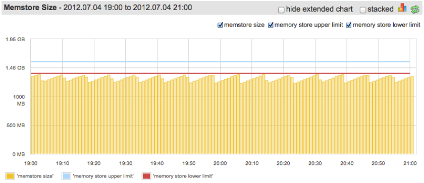
Hint: watch for Memstore Size and Memstore Flush Queue size. Memstore Size ideally should not reach upper Memstore limit and Memstore Flush Queue size should not constantly grow.

Frequent Memstore Flushes

Since we want to avoid blocking writes it may seem a good approach to flush earlier when we are far from “writes-blocking” thresholds. However, this will cause too frequent flushes which can affect read performance and bring additional load to the cluster.

Every time Memstore flush happens one HFile created for each CF. Frequent flushes may create tons of HFiles. Since during reading HBase will have to look at many HFiles, the read speed can suffer.

To prevent opening too many HFiles and avoid read performance deterioration there’s HFiles compaction process. HBase will periodically (when certain configurable thresholds are met) compact multiple smaller HFiles into a big one. Obviously, the more files created by Memstore flushes, the more work (extra load) for the system. More to that: while compaction process is usually performed in parallel with serving other requests, when HBase cannot keep up with compacting HFiles (yes, there are configured thresholds for that too;)) it will block writes on RS again. As mentioned above, this is highly undesirable.

Hint: watch for Compaction Queue size on RSs. In case it is constantly growing you should take actions before it will cause problems.

More on HFiles creation & Compaction can be found here.

So, ideally Memstore should use as much memory as it can (as configured, not all RS heap: there are also in-memory caches), but not cross the upper limit. This picture (screenshot was taken from our SPM monitoring service) shows somewhat good situation:

Memstore Size: Good Situation

“Somewhat”, because we could configure lower limit to be closer to upper, since we barely ever go over it.

Multiple Column Families & Memstore Flush

Memstores of all column families are flushed together (this might change). This means creating N HFiles per flush, one for each CF. Thus, uneven data amount in CF will cause too many HFiles to be created: when Memstore of one CF reaches threshold all Memstores of other CFs are flushed too. As stated above too frequent flush operations and too many HFiles may affect cluster performance.

Hint: in many cases having one CF is the best schema design.

HLog (WAL) Size & Memstore Flush

On RegionServer write/read paths picture above you may also noticed a Write-ahead Log (WAL) where data is getting written by default. It contains all the edits of RegionServer which were written to Memstore but were not flushed into HFiles. As data in Memstore is not persistent we need WAL to recover from RegionServer failures. When RS crushes and data which was stored in Memstore and wasn’t flushed is lost, WAL is used to replay these recent edits.

When WAL (in HBase it is called HLog) grows very big, it may take a lot of time to replay it. For that reason there are certain limits for WAL size, which when reached cause Memstore to flush. Flushing Memstores decreases WAL as we don’t need to keep in WAL edits which were written to HFiles (persistent store). This is configured by two properties: hbase.regionserver.hlog.blocksize and hbase.regionserver.maxlogs. As you probably figured out, maximum WAL size is determined by hbase.regionserver.maxlogs * hbase.regionserver.hlog.blocksize (2GB by default). When this size is reached, Memstore flushes are triggered. So, when you increase Memstore size and adjust other Memstore settings you need to adjust HLog ones as well. Otherwise WAL size limit may be hit first and you will never utilize all the resources dedicated to Memstore. Apart from that, triggering of Memstore flushes by reaching WAL limit is not the best way to trigger flushing, as it may create “storm” of flushes by trying to flush many Regions at once when written data is well distributed across Regions.

Hint: keep hbase.regionserver.hlog.blocksize * hbase.regionserver.maxlogs just a bit above hbase.regionserver.global.memstore.lowerLimit * HBASE_HEAPSIZE.

Compression & Memstore Flush

With HBase it is advised to compress the data stored on HDFS (i.e. HFiles). In addition to saving on space occupied by data this reduces the disk & network IO significantly. Data is compressed when it is written to HDFS, i.e. when Memstore flushes. Compression should not slow down flushing process a lot, otherwise we may hit many of the problems above, like blocking writes caused by Memstore being too big (hit upper limit) and such.

Hint: when choosing compression type favor compression speed over compression ratio. SNAPPY showed to be a good choice here.


[UPDATE 2012/07/23: added notes about HLog size and Compression types]


Plug: if this sort of stuff interests you, we are hiring people who know about Hadoop, HBase, MapReduce…

@abaranau

HBase Real-time Analytics & Rollbacks via Append-based Updates (Part 2)

This is the second part of a 3-part post series in which we describe how we use HBase at Sematext for real-time analytics with an append-only updates approach.

In our previous post we explained the problem in detail with the help of example and touched on the suggested solution idea. In this post we will go through solution details as well as briefly introduce the open-sourced implementation of the described approach.

Suggested Solution

Suggested solution can be described as follows:

  1. replace update (Get+Put) operations at write time with simple append-only writes
  2. defer processing updates to periodic compaction jobs (not to be confused with minor/major HBase compaction)
  3. perform on the fly updates processing only if user asks for data earlier than updates compacted

Before (standard Get+Put updates approach):

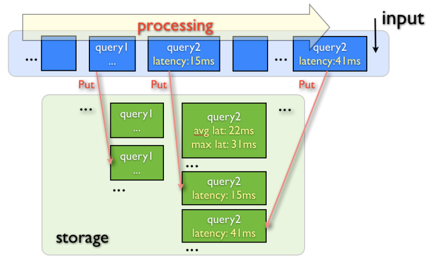
The picture below shows an example of updating search query metrics that can be collected by Search Analytics system (something we do at Sematext).

  • each new piece of data (blue box) is processed individually
  • to apply update based on the new piece of data:
    • existing data (green box) is first read
    • data is changed and
    • written back

After (append-only updates approach):

1. Writing updates:

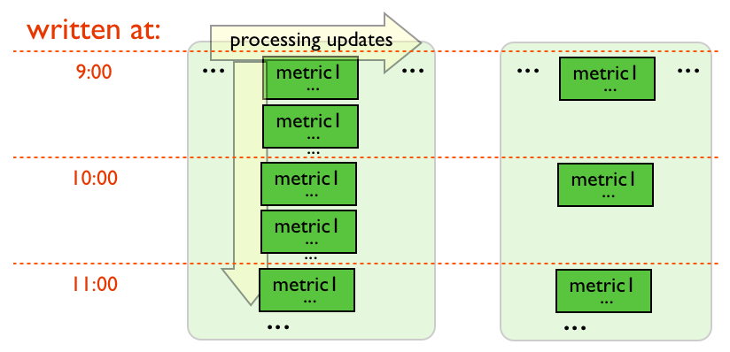
2. Periodic updates processing (compacting):

3. Performing on the fly updates processing (only if user asks for data earlier than updates compacted):

Note: the result of the processing updates on the fly can be optionally stored back right away, so that next time same data is requested no compaction is needed.

The idea is simple and not a new one, but given the specific qualities of HBase like fast range scans and high write throughput it works especially well with HBase. So, what we gain here is:

  • high update throughput
  • real-time updates visibility: despite deferring the actual updates processing, user always sees the latest data changes
  • efficient updates processing by replacing random Get+Put operations with processing sets of records at a time (during the fast scan) and eliminating redundant Get+Put attempts when writing the very first data item
  • better handling of update load peaks
  • ability to roll back any range of updates
  • avoid data inconsistency problems caused by tasks that fail after only partially updating data in HBase without doing rollback (when using with MapReduce, for example)
Let’s take a closer look at each of the above points.

High Update Throughput

Higher update throughput is achieved by not doing Get operation for every record update. Thus, Get+Put operations are replaced with Puts (which can be further optimized by using client-side buffer), which are really fast in HBase. The processing of updates (compaction) is still needed to perform the actual data merge, but it is done much more efficiently than doing Get+Put for each update operation (see below more details).

Real-time Updates Visibility

Users always see latest data changes. Even if updates have not yet been processed and still stored as a series of records, they will be merged on the fly.

By doing periodic merges of appended records we ensure data that has to be processed on the fly is small enough and does fast.

Efficient Updates Processing

  • N Get+Put operations at write time are replaced with N Puts + 1 Scan (shared) + 1 Put operations
  • Processing N changes at once is usually more effective than applying N individual changes

Let’s say we got 360 update requests for the same record: e.g. record keeps track of some sensor value for 1 hour interval and we collect data points every 10 seconds. These measurements needs to be merged in a single record that represents the whole 1-hour interval. Initially we would perform 360 Get+Put operations (while we can use some client-side buffer to perform partial aggregation and reduce the number of actual Get+Put operations, we want data to be sent immediately as it arrives instead of asking user to wait 10*N seconds). With append-only approach, we will perform 360 Put operations, 1 scan (which is actually meant to process not only these updates) that goes through 360 records (stored in sequence), it calculates resulting record, and performs 1 Put operation to store the result back. Fewer operations means using less resources and this leads to more efficient processing. Moreover, if the value which needs to be updated is a complex one (needs time to load in memory, etc.) it is much more efficient to apply all updates at once than one by one individually.

Deferring processing of updates is especially effective when large portion of operations is in essence insertion of new data, but not an update of stored data. In this case a lot of Get operations (checking if there’s something to update) are redundant.

Better Handling of Update Load Peaks

Deferring processing of updates helps handle load peaks without major performance degradation. The actual (periodic) processing of updates can be scheduled for off-peak time (e.g. nights or weekends).

Ability to Rollback Updates

Since updates don’t change the existing data (until they are processed) rolling back is easy.

Preserving rollback ability even after updates were compacted is also not hard. Updates can be grouped and compacted within time periods of given length as shown in the picture below. That means the client that reads data will still have to merge updates on-the-fly even right after compaction is finished. However using the proper configuration this isn’t going to be a problem as the number of records to be merged on the fly will be small enough.

Consider the following example where the goal is to keep all-time avg value for particular sensor. Let’s say data is collected every 10 seconds for 30 days, which gives 259200 separately written data points. While compacting on-the-fly this amount of values might be quite fast for a medium-large HBase cluster, performing periodic compaction will improve reading speed a lot. Let’s say we perform updates processing every 4 hours and use 1 hour interval as compacting base (as shown in the picture above). This gives us, at any point in time, less than 24*30 + 4*60*6 = 2,160 non-compacted records that need to be processed on-the-fly when fetching resulting record for 30 days. This is a small number of records and can be processed very fast. At the same time it is possible to perform rollback to any point in time with 1 hour granularity.

In case system should store more historical data, but we don’t care about rolling it back (if nothing wrong was found during 30 days the data is likely to be OK) then compaction can be configured to process all data older than 30 days as one group (i.e. merge into one record).

Automatic Handling of Task Failures which Write Data to HBase

Typical scenario: task updating HBase data fails in the middle of writing – some data was written, some not. Ideally we should be able to simply restart the same task (on the same input data) so that new one performs needed updates without corrupting data because some write operations were duplicate.

In the suggested solution every update is written as a new record. In order to make sure that performing the same (literally the same, not just similar) update operation multiple times does not result in multiple separate update operations, in which case data will be corrupted, every update operation should write to the record with the same row key from any task attempts. This results in overriding the same single record (if it was created by failed task) and avoiding doing the same update multiple times which in turn means that data is not corrupted.

This especially convenient in situations when we write to HBase table from MapReduce tasks, as MapReduce framework restarts failed tasks for you. With the given approach we can say that handling task failures happens automatically – no extra effort to manually roll back previous task changes and starting a new task is needed.

Cons

Below are the major drawbacks of the suggested solution. Usually there are ways to reduce their effect on your system depending on the specific case (e.g. by tuning HBase appropriately or by adjusting parameters involved in data compaction logic).

  • merging on the fly takes time. Properly configuring periodic updates processing is a key to keeping data fetching fast.
  • when performing compaction, scanning of many records that don’t need to be compacted can happen (already compacted or “alone-standing” records). Compaction can usually be performed only on data written after the previous compaction which allows to use efficient time-based filters to reduce the impact here.

Solving these issues may be implementation-specific. We’ll bring them up again when talking about our implementation in the follow up post.

Implemenation: Meet HBaseHUT

Suggested solution was implemented and open-sourced as HBaseHUT project. HBaseHUT will be covered in the follow up post shortly.


If you like this sort of stuff, we’re looking for Data Engineers!

HBase Real-time Analytics & Rollbacks via Append-based Updates

In this part 1 of a 3-part post series we’ll describe how we use HBase at Sematext for real-time analytics and how we can perform data rollbacks by using an append-only updates approach.

Some bits of this topic were already covered in Deferring Processing Updates to Increase HBase Write Performance and some were briefly presented at BerlinBuzzwords 2011 (video). We will also talk about some of the ideas below during HBaseCon-2012 in late May (see Real-time Analytics with HBase). The approach described in this post is used in our production systems (SPM & SA) and the implementation was open-sourced as HBaseHUT project.

Problem we are Solving

While HDFS & MapReduce are designed for massive batch processing and with the idea of data being immutable (write once, read many times), HBase includes support for additional operations such as real-time and random read/write/delete access to data records. HBase performs its basic job very well, but there are times when developers have to think at a higher level about how to utilize HBase capabilities for specific use-cases.  HBase is a great tool with good core functionality and implementation, but it does require one to do some thinking to ensure this core functionality is used properly and optimally. The use-case we’ll be working with in this post is a typical data analytics system where:

  • new data are continuously streaming in
  • data are processed and stored in HBase, usually as time-series data
  • processed data are served to users who can navigate through most recent data as well as dig deep into historical data

Although the above points frame the use-case relatively narrowly, the approach and its implementation that we’ll describe here are really more general and applicable to a number of other systems, too. The basic issues we want to solve are the following:

  • increase record update throughput. Ideally, despite high volume of incoming data changes can be applied in real-time . Usually. due to the limitations of the “normal  HBase update”, which requires Get+Put operations, updates are applied using batch-processing approach (e.g. as MapReduce jobs).  This, of course, is anything but real-time: incoming data is not immediately seen.  It is seen only after it has been processed.
  • ability to roll back changes in the served data. Human errors or any other issues should not permanently corrupt data that system serves.
  • ability to fetch data interactively (i.e. fast enough for inpatient humans).  When one  navigates through a small amount of recent data, as well as when selected time interval spans years, the retrieval should be fast.

Here is what we consider an “update”:

  • addition of a new record if no records with same key exists
  • update of an existing record with a particular key

Let’s take a look at the following example to better understand the problem we are solving.

Example Description

Briefly, here are the details of an example system:

  • System collects metrics from a large number of sensors (N) very frequently (each second) and displays them on chart(s) over time
  • User needs to be able to select small time intervals to display on a chart (e.g. several minutes) as well as very large spans (e.g. several years)
  • Ideally, data shown to user should be updated in real-time (i.e. user can see the most recent state of the sensors)

Note that even if some of the above points are not applicable to your system the ideas that follow may still be relevant and applicable.

Possible “direct” Implementation Steps

The following steps are by no means the only possible approach.

Step 1: Write every data point as a new record or new column(s) in some record in HBase. In other words, use a simple append-only approach. While this works well for displaying charts with data from short time intervals, showing a year (there are about 31,536,000 seconds in one year) worth of data may be too slow to call the experience “interactive”.

Step 2: Store extra records with aggregated data for larger time intervals (say 1 hour, so that 1 year = 8,760 data points). As new data comes in continuously and we want data to be seen in real-time, plus we cannot rely on data coming in a strict order, say because one sensor had network connectivity issues or we want to have ability to import historical data from a new data source, we have to use update operations on those records that hold data for longer intervals. This requires a lot of Get+Put operations to update aggregated records and this means degradation in performance — writing to HBase in this fashion will be significantly slower compared to using the append-only approach described in Step 1. This may slow writes so much that a system like this may not actually be able to keep up with the volume of the incoming data.  Not good.

Step 3: Compromise real-time data analysis and process data in small batches (near real-time). This will decrease the load on HBase as we can process (aggregate) data more efficiently in batches and can reduce the number of update (Get+Put) operations. But do we really want to compromise real-time analytics? No, of course not.  While it may seem OK in this specific example to show data for bigger intervals with some delay (near real-time), in real-world systems this usually affects other charts/reports, such as reports that need to show total, up to date figures. So no, we really don’t want to compromise real-time analytics if we don’t have to. In addition, imagine what happens if something goes wrong (e.g. wrong data was fed as input, or application aggregates data incorrectly due to a bug or human error).  If that happens we will not be able to easily roll back recently written data. Utilizing native HBase column versions may help in some cases, but in general, when we want greater control over rollback operation a better solution is needed.

Use Versions for Rolling Back?

Recent additions in managing cell versions make cell versioning even more powerful than before. Things like HBASE-4071 make it easy to store historical data without big data overhead by cleaning old data efficiently. While it seems obvious to use versions (native HBase feature) for allowing rolling back data changes, we cannot (and do not want to) rely heavily on cell versions here. The main reason for that is that it is just not very effective when dealing with lots of versions for a given cell. When update history for a record/cell becomes very long this requires many versions for a given cell. Versions are managed and navigated as a simple list in HBase (as opposed to using a Map-like structure that is used for records and columns) so managing long lists of versions is less efficient than having a bunch of separate records/columns. Besides, using versions will not help us with Get+Put situation and we are aiming to kill these two birds with one rock with the solution we are about to describe. One could try to use append-only updates approach described below and use cells versions as update log, but this would again bring us to managing long lists in a non-efficient way.

Suggested Solution

Given the example above, our suggested solution can be described as follows:

  • replace update (Get+Put) operations at write time with simple append-only writes and defer processing of updates to periodic jobs or perform aggregations on the fly if user asks for data earlier than individual additions are processed.

The idea is simple and not necessarily novel, but given the specific qualities of HBase, namely fast range scans and high write throughput, this approach works very well.  So well, in fact, that we’ve implemented it in HBaseHUT and have been using it with success in our production systems (SPM & SA).

So, what we gain here is:

  • high update throughput
  • real-time updates visibility: despite deferring the actual updates processing, user always sees the latest data changes
  • efficient updates processing by replacing random Get+Put operations with processing whole sets of records at a time (during the fast scan) and eliminating redundant Get+Put attempts when writing first data item
  • ability to roll back any range of updates
  • avoid data inconsistency problems caused by tasks that fail after only partially updating data in HBase without doing rollback (when using with MapReduce, for example)

In part 2 post we’ll dig into the details around each of the above points and we’ll talk more about HBaseHUT, which makes all of the above possible. If you like this sort of stuff, we’re looking for Data Engineers!

HBaseWD: Avoid RegionServer Hotspotting Despite Sequential Keys

In HBase world, RegionServer hotspotting is a common problem.  We can describe this problem with a single sentence: while writing records with sequential row keys allows the most efficient reading of data range given the start and stop keys, it causes undesirable RegionServer hotspotting at write time. In this 2-part post series we’ll discuss the problem and show you how to avoid this infamous problem.

Problem Description

Records in HBase are sorted lexicographically by the row key. This allows fast access to an individual record by its key and fast fetching of a range of data given start and stop keys. There are common cases where you would think row keys forming a natural sequence at write time would be a good choice because of  types of queries that will fetch the data later. For example, we may want to associate each record with a timestamp so that later we can fetch records from a particular time range.  Examples of such keys are:

  • time-based format: Long.MAX_VALUE – new Date().getTime()
  • increasing/decreasing sequence: ”001”, ”002”, ”003”,… or ”499”, ”498”, ”497”, …

But writing records with such naive keys will cause hotspotting because of how HBase writes data to its Regions.

RegionServer Hotspotting

When records with sequential keys are being written to HBase all writes hit one Region.  This would not be a problem if a Region was served by multiple RegionServers, but that is not the case – each Region lives on just one RegionServer.  Each Region has a pre-defined maximal size, so after a Region reaches that size it is split in two smaller Regions.  Following that, one of these new Regions takes all new records and then this Region and the RegionServer that serves it becomes the new hotspot victim.  Obviously, this uneven write load distribution is highly undesirable because it limits the write throughput to the capacity of a single server instead of making use of multiple/all nodes in the HBase cluster. The uneven load distribution can be seen in Figure 1. (chart courtesy of SPM for HBase):

HBase RegionServer Hotspotting
Figure 1. HBase RegionServer hotspotting

We can see that while one server was sweating trying to keep up with writes, others were “resting”. You can find some more information about this problem in HBase Reference Guide.

Solution Approach

So how do we solve this problem?  The cases discussed here assume that we don’t have all data we want to write to HBase all at once, but rather that the data are arriving continuously. In case of bulk import of data into HBase the best solutions, including those that avoid hotspotting, are described in bulk load section of HBase documentation.  However, if you are like us at Sematext, and many organizations nowadays are, the data keeps streaming in and needs processing and storing. The simplest way to avoid single RegionServer hotspotting in case of continuously arriving data would be to simply distribute writes over multiple Regions by using random row keys. Unfortunately, this would compromise ability to do fast range scans using start and stop keys. But that is not the only solution.  The following simple approach solves the hotspotting issue while at the same time preserving the ability to fetch data by start and stop key.  This solution, mentioned multiple times on HBase mailing lists and elsewhere is to salt row keys with a prefix.  For example, consider constructing the row key using this:

new_row_key = (++index % BUCKETS_NUMBER) + original_key

For the visual types among us, that may result in keys looking as shown in Figure 2.

HBase Row Key Prefix Salting
Figure 2. HBase row key prefix salting

Here we have:

  • index is the numeric (or any sequential) part of the specific record/row ID that we later want to use for record fetching (e.g. 1, 2, 3 ….)
  • BUCKETS_NUMBER is the number of “buckets” we want our new row keys to be spread across. As records are written, each bucket preserves the sequential notion of original records’ IDs
  • original_key is the original key of the record we want to write
  • new_row_key is the actual key that will be used when writing a new record (i.e. “distributed key” or “prefixed key”). Later in the post the “distributed records” term is used for records which were written with this “distributed key”.

Thus, new records will be split into multiple buckets, each (hopefully) ending up in a different Region in the HBase cluster. New row keys of bucketed records will no longer be in one sequence, but records in each bucket will preserve their original sequence. Of course, if you start writing into an empty HTable, you’ll have to wait some time (depending on the volume and velocity of incoming data, compression, and maximal Region size) before you have several Regions for a table. Hint: use pre-splitting feature for the new table to avoid the wait time.  Once writes using the above approach kick in and start writing to multiple Regions your “slaves load” chart should look better.

HBase RegionServer evenly distributed write load
Figure 3. HBase RegionServer evenly distributed write load

Scan

Since data is placed in multiple buckets during writes, we have to read from all of those buckets when doing scans based on “original” start and stop keys and merge data so that it preserves the “sorted” attribute. That means BUCKETS_NUMBER more Scans and this can affect performance. Luckily, these scans can be run in parallel and performance should not degrade or might even improve — compare the situation when you read 100K sequential records from one Region (and thus one RegionServer) with reading 10K records from 10 Regions and 10 RegionServers in parallel!

Get/Delete

To get or delete a single record by original key may need to perform 1 or up to BUCKETS_NUMBER Get operations depending on the logic we used for prefix generation. E.g. when using “static” hash as prefix, given the original key we may precisely identify the prefixed key. In case we used random prefix we will have to perform Get for each of the possible buckets. The same goes for Delete operations.

MapReduce Input

Since we still want to benefit from data locality, the implementation of feeding “distributed” data to a MapReduce job will likely break the order in which data comes to mappers. This is at least true for the current HBaseWD implementation (see below). Each map task will process data for a particular bucket. Of course, records will be in same order based on original keys within a bucket. However, since two records which were meant to be “near each other” based on their original key may have fallen into different buckets, the will be fed to different map tasks. Thus, if the mapper assumes records come in the strict/original sequence, we will be hurt, since the order will be preserved only within each bucket, but not globally.

Increased Number of Map Tasks

When using data (written using the suggested approach) as a MapReduce input (with start and/or stop key provided) the splits number will likely to be increased (depends on the implementation). For current HBaseWD implementation you’ll get BUCKETS_NUMBER times more splits compared to “regular” MapReduce with same parameters.  This is due to the same logic for data selection as with simple Scan operation, as described above. As the result, MapReduce jobs will have BUCKETS_NUMBER times more map tasks. This should not decrease performance if BUCKETS_NUMBER is reasonably not too high (when MR job initialization & cleanup work takes more time than processing itself). Moreover, in many use-cases having many more mappers helps improve performance. Many users reported more mappers having a positive impact given that standard HTable input based MapReduce job usually has too few map tasks (one per Region) which cannot be changed without extra coding.

Another strong signal the suggested approach and its implementation could help is if in your application, in addition to writing records with sequential keys, the application also continuously processes newly written data delta using MapReduce . In such use-cases when data is written sequentially (not using any artificial distribution) and is being processed relatively frequently, the delta to be processed resides in just a few Regions (or perhaps in even just one Region if the write load is not high, if maximal Region size is high, and processing batches are very frequent).

Solution Implementation: HBaseWD

We implemented the solution described above and open-sourced it as a small HBaseWD project. We say small because HBaseWD is really self-contained and really simple to integrate into an existing code due to support for native HBase client API (see examples below). HBaseWD project was first presented at BerlinBuzzwords 2011(video) and is currently used in a number of production systems.

Configuring Distribution

Simple Even Distribution

Distributing records with sequential keys to be distributed in up to Byte.MAX_VALUE buckets (single byte is added in front of a key):

byte bucketsCount = (byte) 32; // distributing into 32 buckets
RowKeyDistributor keyDistributor =  new RowKeyDistributorByOneBytePrefix(bucketsCount);
Put put = new Put(keyDistributor.getDistributedKey(originalKey));
... // add values
hTable.put(put);

Hash-Based Distribution

Another useful RowKeyDistributor is RowKeyDistributorByHashPrefix. Please see example below. It creates the “distributed key” based on original key value so that later when you have original key and want to update the record you can calculate distributed key without having to call HBase (too see what bucket it is in). Or, you can perform a single Get operation when original key is known (instead of reading from all buckets).

AbstractRowKeyDistributor keyDistributor =
     new RowKeyDistributorByHashPrefix(
            new RowKeyDistributorByHashPrefix.OneByteSimpleHash(15));

You can use your own hashing logic here by implementing this simple interface:

public static interface Hasher extends Parametrizable {
  byte[] getHashPrefix(byte[] originalKey);
  byte[][] getAllPossiblePrefixes();
}

Custom Distribution Logic

HBaseWD is designed to be flexible especially when it comes to supporting custom row key distribution approaches. In addition to the above mentioned ability to implement custom hashing logic to be used with RowKeyDistributorByHashPrefix, one can define custom row key distribution logic by extending AbstractRowKeyDistributor abstract class whose interface is super simple:

public abstract class AbstractRowKeyDistributor implements Parametrizable {
  public abstract byte[] getDistributedKey(byte[] originalKey);
  public abstract byte[] getOriginalKey(byte[] adjustedKey);
  public abstract byte[][] getAllDistributedKeys(byte[] originalKey);
  ... // some utility methods
}

Common Operations

Scan

Performing a range scan over data:

Scan scan = new Scan(startKey, stopKey);
ResultScanner rs = DistributedScanner.create(hTable, scan, keyDistributor);
for (Result current : rs) {
  ...
}

Configuring MapReduce Job

Performing MapReduce job over the data chunk specified by Scan:

Configuration conf = HBaseConfiguration.create();
Job job = new Job(conf, "testMapreduceJob");
Scan scan = new Scan(startKey, stopKey);
TableMapReduceUtil.initTableMapperJob("table", scan,
RowCounterMapper.class, ImmutableBytesWritable.class, Result.class, job);
// Substituting standard TableInputFormat which was set in
// TableMapReduceUtil.initTableMapperJob(...)
job.setInputFormatClass(WdTableInputFormat.class);
keyDistributor.addInfo(job.getConfiguration());

What’s Next?

In the next post we’ll cover:

  • Integration into already running production systems
  • Changing distribution logic in running systems
  • Other “advanced topics”
If you’ve read this far you must be interested in HBase.  And since we (@sematext) are interested in people with interest in HBase, here are some open positions at Sematext, some nice advantages we offer and “problems” we are into that you may want to check out.
Oh, and all HBase performance charts you see in this post are from our SPM service which uses HBase and, you guessed it, HBaseWD too! 😉

Hadoop 1.0.0 – Extra Notes

The big Hadoop 1.0.0 release has arrived.  The general notes about releases from the dev team include:

  • security
  • Better support for HBase (append/hsynch/hflush, and security)
  • webhdfs (with full support for security)
  • performance enhanced access to local files for HBase
  • other performance enhancements, bug fixes, and features

You can also find the complete release notes here and see all fixes, improvements and new features included in the release. To save you time, please find below additional information about some of the items that attracted our attention from the Hadoop 1.0.0 release.

Cluster Management Optimizations

HADOOP-7728hadoop-setup-conf.sh should be modified to enable task memory manager
Adds additional options to manage memory usage by MR tasks. In particular, this allows to set max memory usage for map and reduce tasks (separately).

Performance Improvements

HDFS-2246hadoop-setup-conf.sh should be modified to enable task memory manager
This is a short-term solution for the issue HDFS-347 “DFS read performance suboptimal when client co-located on nodes with data” which is quite hot in Hadoop dev community nowadays. NOTE: by default this optimization is switched off (or is it? Update: it is not, see the comments) so some config adjustments are required to benefit from it. And you will definitely want to benefit from it: some reported two times I/O performance improvements. Also highly recommended for HBase users.

HDFS-895Allow hflush/sync to occur in parallel with new writes to the file
Previously if a hflush/sync were in progress, an application could not write data to the HDFS client buffer. Again we stress out this improvement for HBase users as this increases the write throughput of the transaction log in HBase.

MAPREDUCE-2494Make the distributed cache delete entires using LRU priority
When certain threshold was reached and distributed cache was being purged, previous implementation deleted all entries that were not currently being used. With new code more hot data can be left in the cache (the percentage is configurable) and thus decrease cache misses.

New Features

HDFS-2316 [umbrella] WebHDFS: a complete FileSystem implementation for accessing HDFS over HTTP
Allows accessing HDFS over HTTP (read & write)

MAPREDUCE-3169Create a new MiniMRCluster equivalent which only provides client APIs cross MR1 and MR2
Cleaner MR1 & MR2 compatible API for mini MR cluster to be used in unit-tests.

HADOOP-7710Create a script to setup application in order to create root directories for application such hbase, hcat, hive etc
Similar to hadoop-setup-user script, a hadoop-setup-applications script was added to set up root directories for apps to write to (/hbase, /hive, etc.)

Enjoy Hadoop 1.0.0 and we hope you found this quick summary useful!

@sematext

Flume and HBase Integration

This quick How-To post will teach you how to use HBase sink(s) in Flume. There are currently two generic HBase sinks available: hbase() and attr2hbase(). The former requires one to be more explicit when providing mapping from event data to HBase record, while the latter allows adding record cells dynamically based on event data. Despite this difference, these two sinks have a lot in common.

Configuring Sink(s)

Both sinks write a single or no records into an HBase table based on a single Flume event. Both sinks have three attributes (at least) in common: table, writeBufferSize and writeToWal. These attributes control the HBase client behavior.

The attribute table is the name of the output HBase table. Yes, that means that currently one sink can be configured to output into just one table. If you desperately need to write to multiple tables you can use Flume’s native features to configure several sinks and direct each to the desired HBase table.

The writeBufferSize corresponds to the attribute of HTable with the same name and defines client-side buffer (in bytes). If writeBufferSize has a non-zero value, the HTable’s autoFlush is set to false. In this case the sink buffers data and sends them in chunks of the writeBufferSize size to the server.  This decreases the number of remote invocations and helps improve performance. By default the sink sends data on every received event. While it seems obvious that one would want to specify a bigger buffer to improve performance, determining the best buffer size depends on the use-case: no data will be sent to server before the buffer is full, which may break some “near real-time” models. The default writeBufferSize for HTable is 2 MB. Another important factor to consider is that the greater client-side buffer you have the more data you might loose in case of HBase failure [11]. Please find more details about this in Reliability Issues part of this post.

The writeToWal corresponds to the attribute of the HBase Put with the same name. If set to false the Put operations will not be written into HBase’s edit log. While this means fewer operations to perform and hence much better performance, this approach isn’t reliable: every non-persistent change (HBase likes to keep as much data as it can in memory to keep things fast) will be lost in case of HBase failure [1]. One would typically want to skip writing edits to WAL in case losing some portion of data is acceptable (e.g. when doing non mission-critical log analysis) or during a bulk import (it goes  much faster without writing to WAL) which can be restarted in case of failure.

HBase Sink: hbase()

As of this writing the hbase() sink has the following semantics:

hbase("table", "rowkey", "cf1", "c1", "val1"[,"cf2", "c2", "val2", ....]
 {, writeBufferSize=int, writeToWal=true|false})

As you can see, one is asked to provide the values to be placed into the HBase record explicitly. One has to use expressions in values of “rowkey”, “cf1”, “c1”, “val1”, etc. to make it usable. Expressions available with any event type are “%{hostname}” (or “%{host}”), “%{nanos}”, “%{priority}”, “%{body}” (and soon “%{timestamp}” [8]) which resolve to event properties. You can also fetch value of any event’s custom attribute with the help of “%{attribute_name}”. For example, with the following configuration an HBase table would be populated with records so that one record corresponds to one event with event’s nanos (event.getNanos()) as row key and two cells in event_colfam column family: body and host with values of event’s body and hostname respectively.

hbase("table", "%{nanos}", "event_colfam", "body", "%{body}",
      "event_colfam", "host", "%{host}")

HBase Sink: attr2hbase()

This sink was originally contributed to Flume by Sematext, as we needed it for our products that make use of Flume and HBase.

As of this writing the attr2hbase() has the following semantic:

attr2hbase("table"[,"sysFamily"[,"writeBody"[,"attrPrefix"[,"writeBufferSize"
 [,"writeToWal"]]]]])

The attr2hbase() sink is used to write event attributes that correspond to a particular format (name starts with a specified prefix) into an HBase record. The names of columns (qualifiers) and column families are determined dynamically based on event’s attribute names. Thus, compared to the hbase() sink, you don’t have to list all possible event attributes you want to store in HBase along with their destination column families and qualifiers (columns). Your source and/or decorators can produce any (reasonable) number of attributes, with dynamic names (e.g. depending on the values) and they will be written into HBase if attr2hbase() sink is configured correctly. In other words, with attr2hbase() one can a) define column names at run-time and b) add whatever number of columns the business logic requires (also at run-time, based on the data being processed). E.g. in case email messages are processed we can store each recipient in a separate cell in an HBase record. You may want to implement your own decorator for that (keep reading to learn how to do this) due to some limitations [9].

sysFamily holds the name of the column family that  is used to store “system” data (event timestamp, host, priority). In case this parameter is absent or equals “”, the sink doesn’t write “system” data. E.g. with configuration like this:

attr2hbase( "mytable", "sysColfam")

each record will have the following cells:

sysColFam:timestamp=<event’s timestamp>, sysColFam:host=<event’s host>, sysColFam:priority=<event’s prioirty>:

hbase(main):002:0> scan 'mytable'         
ROW    COLUMN+CELL                                                                                                              
 123   column=sysColfam:host, timestamp=1309275728725, value=testhost                                        
 123   column=sysColfam:priority, timestamp=1309275728725, value=INFO                                                           
 123   column=sysColfam:timestamp, timestamp=1309275728725, value=\x00\x00\x010\xD6\xEA+T

writeBody indicates whether event body should be written with other “system” data. By default, (when this parameter is absent or equals ””) the attribute body is not written. This parameter should have the “column-family:qualifier” format in order for the sink to write the body to the specific column-family:qualifier.

attrPrefix defines which attributes will be written to HBase: every attribute with the name prefixed with attrPrefix parameter’s value is written.  The attribute key should be in the following format to be properly written into HBase:

“<attrPrefix><colfam>:<qual>”

The default value of attrPrefix is “2hb_”.  This means that all attributes with names “2hb_<colfam>:<qual>” should be written to HBase. Attribute with key “<attrPrefix>” must contain row key for Put, otherwise, if no row can be extracted, the event is skipped and no record is written to the HBase table. The table below shows how event attributes are handled: each cell shows where the event attribute  (first column) will be written based on the sink parameters (second and other cells in table header).

Event’s attr (“name”->”value”) attrPrefix=”2hb_”, sysFamily=null attrPrefix=”2hb_”, sysFamily=”sysfam” attrPrefix=””, sysFamily=”sysfam” attrPrefix=””, sysFamily=null
“any”->”foo” sysfam:any->foo
“colfam:col”->”foo” colfam:col->foo colfam:col->foo
“2hb_any”->”foo” sysfam:any->foo sysfam:2hb_any->foo
“2hb_colfam:col”->”foo” colfam:col->foo colfam:col->foo 2hb_colfam:col->foo 2hb_colfam:col->foo

Example

This sink is usually used with the decorators that perform light transformation of event data into attributes with specific names. We say “light transformation” here to avoid getting into the discussion about whether Flume is meant for ETL or just for reliable data delivery. You can use different standard Flume decorators [2], like “value()”, “select()”, “regex()”, “split()” and others. For example, the following setting will make Flume write a new record into HBase table for every line in a tailed file:

'tail("/tmp/some.log")'
'split( ":", 0 , "2hb_colfam:ts")
 split( ":", 1 ,"2hb_colfam:value")
 format("%{nanos}:") split(":", 0, "2hb_")
  attr2hbase( "mytable", "", "", "2hb_", "1000", "false" )'

NOTE: we have to use format() + split() decorators as workaround for FLUME-676 [3]: value() sink doesn’t support EL values. So with format() we put %{nanos} into the body and then from there we put it into attribute with name “2hb_”. The written records will have row key whose value will hold the nanos of the event timestamp (“2hb_” attribute value) and two values pased from log line. Here’s the example output:

$ echo "2238947398:56" >> /tmp/some.log
$ hbase shell
hbase(main):025:0> scan 'mytable'
ROW COLUMN+CELL
9656555664717551 column=colfam:ts, timestamp=1308748686334, value=2238947398
9656555664717551 column=colfam:value, timestamp=1308748686334, value=56

Custom Decorator

The attr2hbase sink is often used with custom decorator that “prepares” events so that they contain attributes ready to be written into an HBase table. Implementing a custom decorator is very simple. Example code:

public class CustomDecorator<S extends EventSink> extends
EventSinkDecorator<S> {
  public CustomDecorator(String param) {
    super(null);
    // TODO: do some initialization
  }

  public void append(Event e) throws IOException {
        // TODO: transform event e here
    super.append(e);
  }

  public static SinkFactory.SinkDecoBuilder builder() {
    return new SinkFactory.SinkDecoBuilder() {
      @Override
      public EventSinkDecorator<EventSink> build(Context context,
          String... argv) {
        if (argv.length != 1) {
          throw new IllegalArgumentException("
usage: CustomDecorator(\"param\")");
        }
                return new CustomDecorator<EventSink>(argv[0]);
      }
    };

  }

  public static List<Pair<String, SinkFactory.SinkDecoBuilder>>
getDecoratorBuilders() {
    return Arrays.asList(new Pair<String,
SinkFactory.SinkDecoBuilder>("CustomDec", builder()));
  }

}

To make your custom decorator visible to Flume you need to register it in flume-site.xml:

<configuration>
<property>
<name>flume.plugin.classes</name>
 <value>your.own.CustomDecorator</value>
</property>
...
</configuration>

Reliability Issues

There are certain reliability details you will want to think about when using HBase sinks.

Temporary HBase Connection Loss Requires Sink Restart

If default HBase configuration is used, when connection from sink node to HBase cluster breaks for several minutes (e.g. network problems or cluster maintenance downtime) the sink stops working. Unfortunately, it does not recover after cluster becomes accessible again. To fix this behavior you can adjust configuration properties “hbase.client.pause” and “hbase.client.retries.number” in hbase-site.xml which should be in Flume’s classpath. The default behavior (i.e. the issue) is going to be fixed in a future release [10].

Loss of Data Buffered on Client-side

Despite using reliable data delivery approaches (like agentE2ESink), there is a loss of data possible if client-side buffer is used (i.e. if writeBufferSize > 0) when failure happens during the buffer flushing [11]. This occurs because the ACK about data being received is sent before the actual write to an HBase table is done – writes are performed only on buffer flush, not on per-event basis. Thus, in case of a write failure during flushing data from the client-side will be lost as ACKs will fool Flume into thinking data have already been persisted in HBase.

Other Considerations

Row Key

As usually, one of the most important design decisions when using HBase is around row key format/values. In initial versions of HBase sinks the default row key was %{nanos}, as it seems to be unique and records seems to be ordered by arrival time. However, we suggest you consider using a different row key value/format, and here’s why. Usually when users import data into HBase they use either some kind of UUID or a timestamp (inverted) based approach. The former helps achieve better performance by distributing write load between multiple regions. The latter is good when one needs fast scans of imported data based on time ranges and when import load is bearable. However, when we use nanos, which are currently obtained from System.nanoTime() Java call, we don’t achieve any of these advantages: keys from each event-producer go in sequence, so all write load is distributed over just a few regions and region servers at a time [12], and System.nanoTime() is not really suitable for use in scans for fetching data from a time interval. Moreover, we cannot even rely on records being written from different Flume nodes being ordered by time of arrival, as nanos are not necessarily in sync across JVMs. Thus, it may make more sense to use pure random row keys (although Flume has no %{random} or anything similar, as far as we know) or a timestamp (inverted) [8] (along with [12] if that is possible). There might be more work needed with timestamp-based approach: there is a possibility to get events with the exact same timestamp during high load. Thus, adding an extra hash would help here (or even using “%{timstamp}%{nanos}”).

Setup Instructions

The easiest way to install Flume is to use CDH3 [4]. Then you need to add flume-plugin-hbasesink jar into flume lib dir. You can compile it from Flume sources [5] or download a compiled jar [6]. You also need to add HBase jar into Flume’s lib dir. It can be downloaded from Maven repositories [7] or copied from your HBase setup dir (so that the jar used on client-side by Flume sink is the same as the one on the server-side, which is important). The last step is to add plugin(s) to Flume’s configuration file (flume-site.xml):

<configuration>
<property>
<name>flume.plugin.classes</name>
 <value>com.cloudera.flume.hbase.HBaseSink,com.cloudera.flume.hbase.Attr2HBaseEventSink</value>
</property>
...
</configuration>

As both HBase and Flume use Zookeeper, it makes sense to share the Zookeeper quorum, too.

If you read this far, you may want to know that we are hiring and are happy users of and contributors to Flume, HBase, and a few other projects.

[1] http://www.larsgeorge.com/2010/01/hbase-architecture-101-write-ahead-log.html

[2] http://archive.cloudera.com/cdh/3/flume/UserGuide/index.html#_flume_sink_decorator_catalog

[3] https://issues.cloudera.org/browse/FLUME-676

[4] https://ccp.cloudera.com/display/CDHDOC/Flume+Installation

[5] https://github.com/abaranau/flume-plugin-hbasesink-compiled

[6] https://github.com/cloudera/flume

[7] e.g. https://repository.cloudera.com/content/groups/public/org/apache/hbase/hbase/

[8] https://issues.cloudera.org/browse/FLUME-688

[9] https://issues.cloudera.org/browse/FLUME-689

[10] https://issues.cloudera.org/browse/FLUME-685

[11] https://issues.cloudera.org/browse/FLUME-390

[12] https://github.com/sematext/HBaseWD
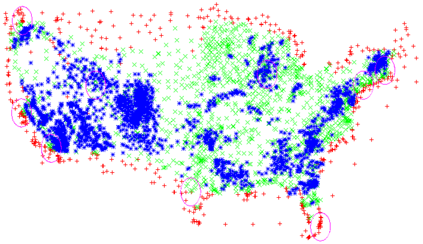
Deferring Processing Updates to Increase HBase Write Performance

In this post we’ll examine, via an example, how deferring the processing of updates can increase write throughput of a data store. In the end we’ll introduce our recently open-sourced HBaseHUT, a tool for automating of deferred updates in HBase.

Please note, that “deferred updates” here does not mean that updates are not “visible” immediately after a write operation. The system still serves add/update/delete and read operations in real-time.

Plug: if this sort of stuff interests you, we are hiring people who know about Hadoop, HBase, MapReduce…

Constraints & Assumptions

The decisions and ideas in the post are based on facts about HBase, but can be applied to many other data stores with similar characteristics:

  • Fetching a set of records as a range (scan operation) is much cheaper than fetching the same records one-by-one
  • Adding new records (simple write operation) is very fast
  • Storage space is cheap
  • “In-place” updates of records are not generally feasible

Well, the last assumption is a bit tricky: HBase provides incrementColumnValue() operation but it is very limited: one can only increment a specified cell that contains long value by some delta. In future versions HBase will allow incrementing of multiple cells at once (already in HBase trunk). However, not all update operations are that simple, as we’ll see in the example. Moreover, incrementing cells in a record is slower than writing a new record (we’ll use this fact later in the post).

Idea Explained

The idea behind deferred updates processing is to postpone updating of the existing record and store incoming deltas as a new record. Thus, record update operations become a simple write operations with corresponding performance. Deferred updates technique elaborated here fits well when system handles a lot of updates of stored data and write performance is the main concern, while reading speed requirements are not that strict. The following cases (each of them separately or any combination of them) may indicate  that one can benefit from using the technique (the list is not complete):

  • updates are well spread over the whole and large dataset
  • lower rate (among write operations) of “true updates” (i.e. low percentage of writes are for completely new data, not really updates of existing data)
  • good portion of data stored/updated may never be accessed
  • system should be able to handle high write peaks without major performance degradation

Next, let’s look at an example use-case to illustrate the idea better.

Example Use-Case

Imagine a simple presentation slides sharing system that gives one the ability to browse presentations on-line (not as downloadable PDF or whatever format files, since that would not be interesting for us here). Suppose we want to provide the presentation’s author with details on user behaviour when a user navigates through slides so that the author can use this data to infer the quality of the presentation (hey, slide sharing systems maintainers: free hint!). Let’s limit statistics data we want to share to simple metrics for the sake of keeping the example simple. Here’s what we can provide:

  • number of times a particular slide was viewed
  • avg/min/max time spent by user on a particular slide

Using these stats the presentation author can find out e.g.:

  • what are the most difficult to understand slides (they probably need to be divided into multiple ones, or better preparation before showing them should be done by giving more/better info on previous slides)
  • what are the most trivial slides (they can be merged/removed)
  • what are the typical users (e.g., If users spend a lot of time thinking on the slides the author can add more details in the presentation.  On the other hand, if users usually quickly walk through it then some very deep details can be removed)

Such a system could provide more stats to authors so that they can work on other sorts of presentation improvements.  For example, the system could provide information about user navigation actions (e.g., if users often go back and forth between two slides then probably the schemes/diagrams on them are better understandable if they are on the same slide and can be easily compared), but that’s not the focus of this post.

To track previously mentioned stats data we need to capture how much time a user spent on a particular slide and send this data to our data store. Let’s assume our records store the following info: {(key)presentationId_slideId, number of views, total viewing time, max viewing time, min viewing time}. Using this data we can provide useful information to author as needed.

Every time user leaves the slide, tracking logic sends the next data to the data store: {(key)presentationId_slideId, time spent on viewing}.

Direct Solution

The straight forward approach would be to update the presentationId_slideId record (fetch, modify and store updated data) as new data comes in. Here are some drawbacks of this naive approach:

  • for each update operation we have to perform fetch and write operations (Get and Put in case of HBase)
  • Most authors won’t really care about all these stats and majority of them will never look at it, so many processing operations can simply be omitted (until there’s interest in stats)
  • for first ever viewing of a slide a redundant fetch operation is performed (data is not there yet), which is OK if slides are viewed many times but in situation when many presentations are viewed just one time (e.g. by their creators) this may result in a bigger portion of redundant operations (this assumption is sort of made up, yes)

The very first point is a major one and is the obvious write performance killer.  This point is really not made up – we have first hand experience with that particular situation.

Deferring Updates Processing

One alternative solution is to defer updates processing to the time when data is requested by presentation author or to the time when the scheduled/periodic updates processing is performed (ideally when data store write load is minimal). In this deferred updates approach all new deltas (new user action data) are written as new records.

When an author requests the stats, efficient updates processing takes place. This time it is done in much more efficient way (compared to direct approach): by using range scan operations, and not by individual record read/writes. Given that presentation has usually tens of slides and is viewed by hundreds or thousands people such range scans are so fast the user will barely notice them. Also, it should be quite OK to ask a person to wait several seconds during his first view of stats page (processed updates are written back into the data store, so next time user fetches data it is available right away).

To prevent too long updates processing on user request the data can be processed periodically instead of at request time. Given the fact that (updated) statistics data is available to user immediately, the processing can be postponed for a long time without affecting the “real-time” visibility aspect of the system. The processing of updates can be scheduled to take place during off-peak hours, when they won’t compromise write performance. By doing this we add a “cushion” since from this point on the maximum amount of data that needs to be processed “on-the-fly” is one day ‘s worth of updates (assuming daily updates processing) , which is sufficient for the majority of cases (e.g. estimated max presentation views per day is tens of thousands which is a very quick scan operation).

The remainder of this post provides details of our implementation of this approach.

HBaseHUT

HBaseHUT is a tool that automates deferred processing of updates for HBase. It hides many details of updates processing from the client code, thus making it an easy to use solution. There are Put and ResultScanner wrappers that encapsulate all needed logic.

To write new data you need to use HutPut implementation of Put. Since it implements the standard HBase Put only the instance creation code needs to be changed:

public class SlideStatsTracker {
  byte[] SLIDE_CF = Bytes.toBytes("slide");
  byte[] VIEWS_NUM_C = Bytes.toBytes("views");
  byte[] TOTAL_VTIME_C = Bytes.toBytes("total_time");
  byte[] MIN_VTIME_C = Bytes.toBytes("min_time");
  byte[] MAX_VTIME_C = Bytes.toBytes("max_time");
  ...
  void trackSlideView(byte[] presentationId, byte[] slideId, long timeSpent)
                               throws InterruptedException, IOException {
    Put put = new HutPut(Bytes.add(presentationId , slideId));
    put.add(SLIDE_CF, VIEWS_NUM_C, Bytes.toBytes(1));
    put.add(SLIDE_CF, TOTAL_VTIME_C, Bytes.toBytes(timeSpent));
    hTable.put(put);
  }
  …
}

Fetching stats is performed using HutResultScanner which implements ResultScanner and hence can also be very easily integrated into the code that uses normal HBase API:

  Scan scan = new Scan(presentationId);
  ResultScanner resultScanner =
      new HutResultScanner(hTable.getScanner(scan), updateProcessor);
  Result result = resultScanner.next();
  while (result != null) {
    // fetch data from result object
    result = resultScanner.next();
  }

The updateProcessor passed as parameter encapsulates update operation logic:

  class SlideStatsUpdateProcessor implements UpdateProcessor {
    @Override
    public void process(Iterable records, UpdateProcessingResult processingResult) {
      int viewsNumber = 0;
      long totalViewTime = 0;
      long minViewTime = Long.MAX_VALUE;
      long maxViewTime = Long.MIN_VALUE;
      // Processing records
      for (Result record : records) {
        for (int i = 0; i < 5; i++) {
          int views = Bytes.toInt(record.getValue(SLIDE_CF, VIEWS_NUM_C));
          long totalTime = Bytes.toLong(record.getValue(SLIDE_CF, TOTAL_VTIME_C));
          long minTime = Bytes.toLong(record.getValue(SLIDE_CF, MIN_VTIME_C));
          long maxTime = Bytes.toLong(record.getValue(SLIDE_CF, MAX_VTIME_C));

          viewsNumber += views;
          totalViewTime += totalTime;
          minViewTime = minTime  maxViewTime ? maxTime : maxViewTime;
        }
      }

      processingResult.add(SLIDE_CF, VIEWS_NUM_C, Bytes.toBytes(viewsNumber));
      processingResult.add(SLIDE_CF, TOTAL_VTIME_C, Bytes.toBytes(totalViewTime));
      processingResult.add(SLIDE_CF, MIN_VTIME_C, Bytes.toBytes(minViewTime));
      processingResult.add(SLIDE_CF, MAX_VTIME_C, Bytes.toBytes(maxViewTime));
    }
  }

As you one can see, HBaseHUT abstraction doesn’t change HBase API and that makes it very easy to use in new code or integrate it in old code.

You can find more details about HBaseHUT features on the project’s wiki. HBaseHUT is a new, recently emerged project – your feedback/questions/ideas/feature requests/forks/pull requests, etc. are all very welcome. Please start new discussions on HBaseHUT’s mailing list.

If you read this far, we’d like to talk to you – we are hiring smart people who know about Hadoop, HBase, MapReduce, want to do large scale data (stream) processing, and build tools like HBaseHUT.